04 — Publications / Explainer
Near harvest, the AI looked
at the grain heads to predict yield
Matching the light and the image size to the growth stage made predictions more accurate
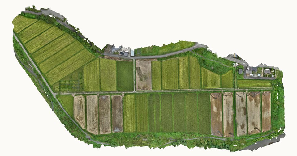
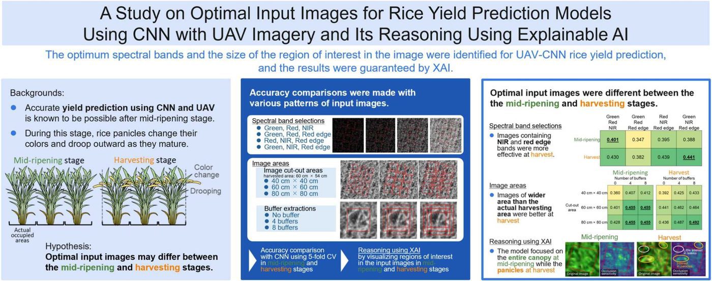
We use drone images of paddy fields and artificial intelligence (AI) to predict how much rice a field will yield. Here we changed when the images were taken, which kinds of light they contained, and how much area each one covered, to find the combination that predicts most accurately. Near harvest, the best results came from light that included red edge and from cutting out each image a little wider than the harvested patch. Maps of where the AI looked showed that it focused on the grain heads (panicles) near harvest, which explains these results.
Key points
- The best combination of light depended on when the images were taken. Near harvest, the combination of green, near-infrared, and red edge light gave the most accurate predictions.
- Cutting out each image a little wider than the patch we harvested made predictions more accurate. The gain was largest for images taken near harvest.
- Maps of where the AI looked showed that it attended to the whole plant at mid-ripening (about three weeks after the panicles appear) and to the panicles near harvest. This difference explains the first two findings.
Why predict rice yield with drones and AI?
Rice is the world's most consumed staple food crop. Knowing how much rice a field will produce, its yield, matters for farmers' decisions and for national planning.
Drones are now widely used to estimate yield. They can photograph fields in fine detail whenever needed, which is especially useful in Japan, where fields are small and the weather is often cloudy or rainy.
For predicting yield from images, a widely used AI is the convolutional neural network (CNN), a type of deep learning that finds useful image features on its own.
Rice changes quickly as it ripens
After heading, when the panicles (the grain-bearing heads) emerge, the grains gradually fill. This period is called ripening. Earlier drone and CNN studies found that images from mid-ripening onward give more accurate and stable predictions.
Yet the plants keep changing as harvest approaches. The grains fill and the panicles turn golden, while the leaves begin to wither. The heavier panicles droop into the gaps between plants and beyond (Figure 1).
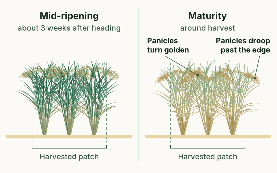
So the most useful light, and how much area each image should include, may depend on when the images are taken. These input image conditions had not been studied in detail.
Another challenge is that it is hard to see why an AI gives a particular answer. Methods that reveal the reasons behind an answer in a form people can understand are called explainable AI (XAI). In agricultural science, XAI had almost never been used with CNNs that predict numbers such as yield.
We therefore compared input image conditions and used XAI to look for the reasons behind the differences. We expected the AI to rely on the whole plant at mid-ripening and on the panicles near harvest.
Three years of images and yields, compared under many conditions
Fields and yield data
We ran the trials from 2021 to 2023 in farmers' paddy fields in Tomioka, Futaba District, Fukushima Prefecture, Japan. In 37 fields covering about 0.9 hectares, we grew five varieties used in the area. They were Fukuhibiki, Fukunoka, Gohyakugawa, Sakurafukuhime, and Tennotsubu.
We measured yield in small patches of six hills (two rows of three), each 60 cm × 54 cm. A hill is a clump of rice plants growing together. We harvested each patch, dried the plants in a plastic greenhouse, threshed them, and divided the grain weight by the patch area.
Over three years we collected yields from 2,184 patches. They ranged from 1.3 to 13.4 metric tons per hectare, a very wide spread.
Drone images
The drone carried a multispectral camera, which records light separately for each color, or wavelength. It can also capture near-infrared (NIR) light, which our eyes cannot see. We used green, red, red edge, and NIR light. Red edge is the narrow band between red and near-infrared.
We flew at two stages, at mid-ripening (about three weeks after heading and two weeks before harvest) and at maturity (around harvest). On sunny days the drone flew 30 or 50 meters above the ground, and we stitched its photos into one map-like image with accurate positions, called an orthoimage. Each pixel covers about 2 cm of ground.
What the AI saw
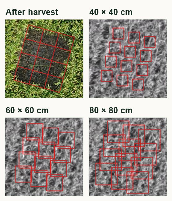
We located each harvested patch in a drone photo taken right after harvest. We then cut a square out of the drone image, centered on each patch, and showed it to the AI (Figure 2).
Each square stacked three of the four kinds of light, just as an ordinary color photo stacks red, green, and blue.
The AI that predicts yield
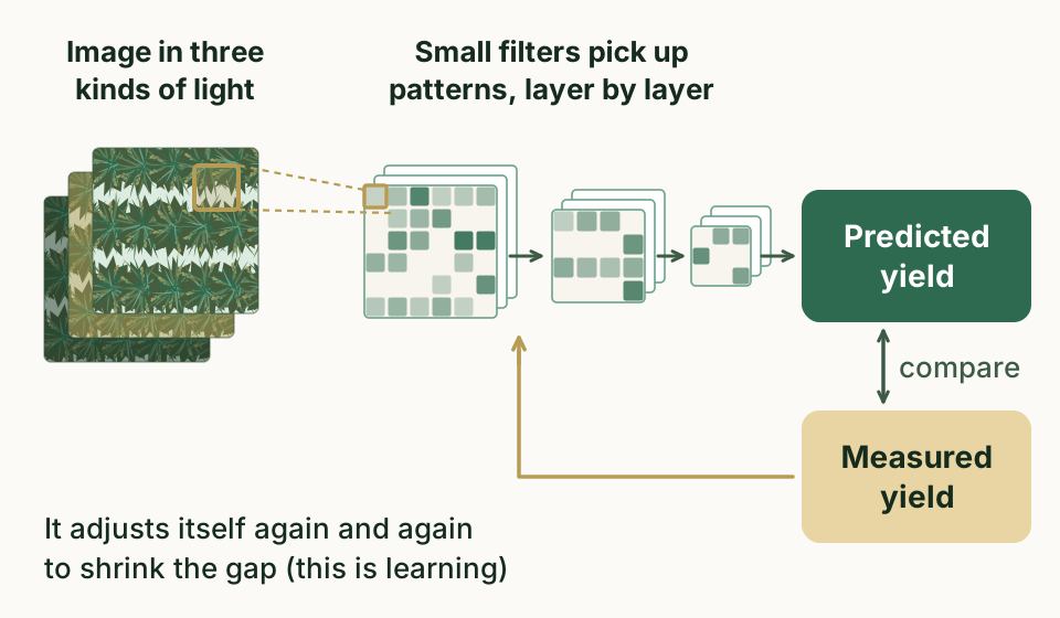
We used a CNN for the predictions. A CNN slides small filters across an image to pick up patterns, then combines them layer by layer until it outputs a single number, the yield (Figure 3).
To train it, we showed it many images paired with the yields measured in the field. Step by step, the CNN adjusts its internal values to shrink the gap between its predictions and those yields. Of the three CNN designs we tried, Xception was the most accurate, so we used it.
We checked accuracy only on patches not used for training. We split the data into groups, trained on all but one, tested on the one left out, and repeated this for each group in turn before averaging the results. This is called cross-validation.
Four conditions we compared
We varied four conditions (Figure 4). The first was timing, mid-ripening or maturity. The second was the light combination. Choosing three of the four kinds gives four options.
The third was the cut-out size. We tried squares 40, 60, and 80 cm on a side, which are smaller than, about equal to, and larger than the 60 cm × 54 cm patch. A wider square might capture more, such as drooping panicles, but it might also take in neighboring plants and confuse the prediction.
The fourth was whether to add shifted copies. We moved the cut-out square by 10 cm and gave the new image the same yield as the original (the paper calls this buffer extraction). We shifted it in 4 directions (up, down, left, and right) or 8 (adding the diagonals), making the training data 5 or 9 times larger.
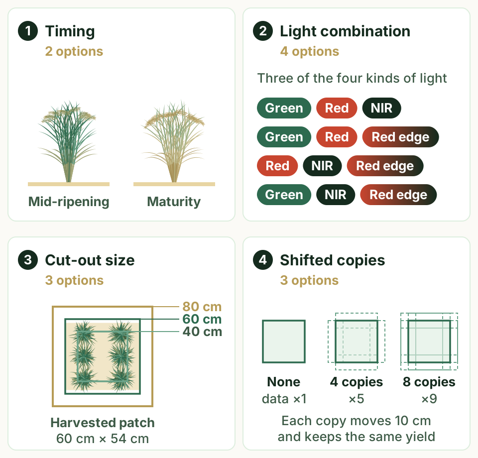
We compared them in two steps. First, we compared the light combinations at each stage. Then, using the best combination for each stage, we compared the cut-out sizes and the numbers of shifted copies.
Gohyakugawa lodged (fell over) across almost the whole field in 2021, so we left out its data from that year. With no mid-ripening images of it from other years, the mid-ripening comparison used the other four varieties.
Seeing where the AI looked
For the most accurate model at each stage, we used two methods to map which parts of the image the AI relied on. Such maps, which show values as colors, are called heat maps.
The first method is occlusion sensitivity. We blank out one spot (set its value to zero), predict again, and see how much the prediction changes. The bigger the change, the more the AI relied on that spot. We repeat this for every spot (Figure 5).
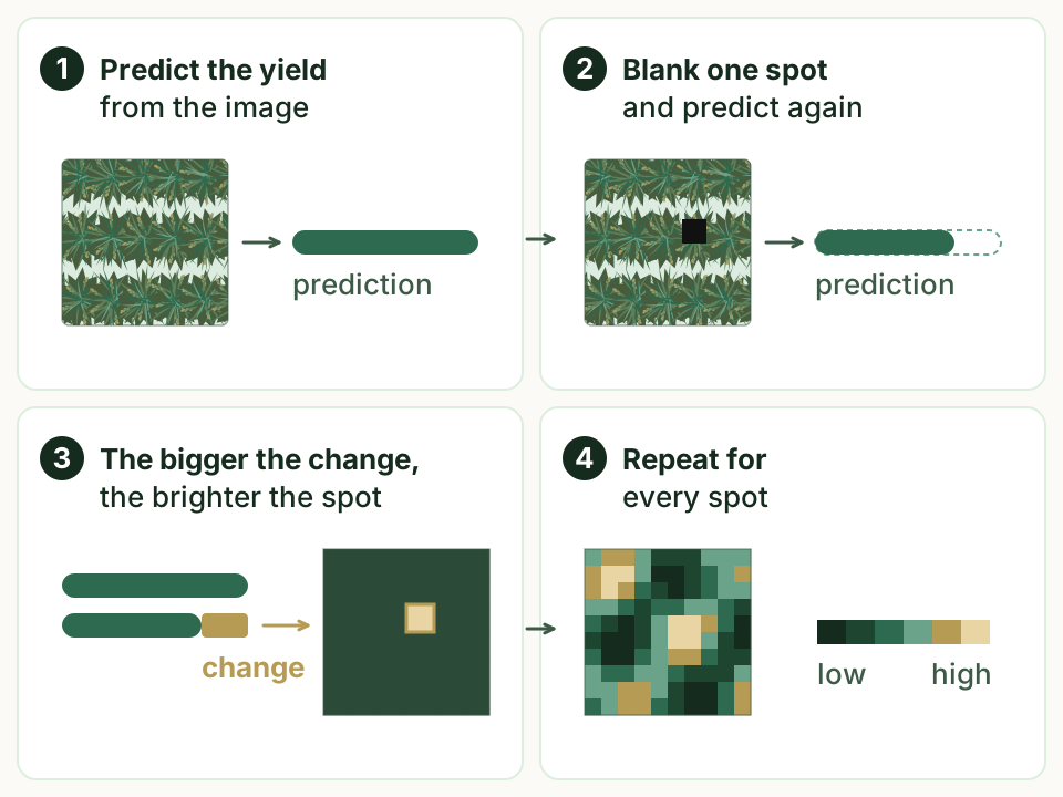
The second is the gradient method. It calculates in one pass how much the prediction would shift if the value at each point changed slightly. We applied both methods to one image per variety at each stage.
The best light and image size depended on the stage
Combinations of light
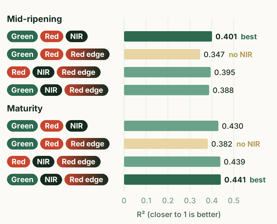
We measured accuracy mainly with the coefficient of determination (R²). It shows how well the predictions match the measured values, and the closer it is to 1, the better.
At mid-ripening, green, red, and NIR gave the most accurate predictions (R² = 0.401). At maturity, green, NIR, and red edge did best (R² = 0.441).
At both stages, the only combination without NIR (green, red, and red edge) gave the lowest values (Figure 6). NIR light is known to track the amount of leaves and the size of the plants well, and it appears to matter for yield prediction too. Red edge was more useful in images taken at maturity.
Cut-out size and shifted copies
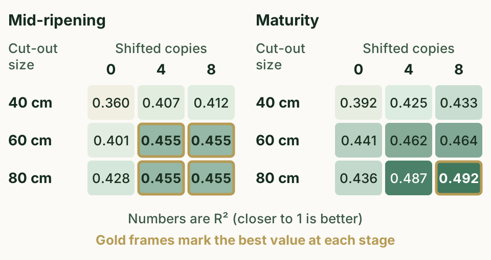
At both stages, accuracy tended to rise as the square got wider and as more shifted copies were added (Figure 7).
At maturity, the widest square (80 cm) with 8 shifted copies was the most accurate. Its R² of 0.492 was the highest in the study, and the typical prediction error was about 15% of the average yield (relative root mean squared error, RRMSE = 0.148).
At mid-ripening, the best results came from 60 or 80 cm squares with 4 or 8 shifted copies, all with an R² of 0.455. The benefit of a wider square was larger at maturity.
In the field, rice plants spread their leaves and panicles beyond the harvested patch. A slightly wider square seems to capture the plants of each patch more fully. Until now, studies have usually cut out images the same size as the harvested area. Showing that a slightly wider cut-out improves accuracy is a new contribution of this study.
Where the AI looked
The heat maps show that at mid-ripening the AI spread its attention evenly over the whole area covered by plants. At maturity, it focused strongly on the panicles, while the leaves showed a mix of spots it attended to and spots it largely ignored (Figure 8).
Both methods showed the same pattern, and it held for every variety, even though flight dates differed by a few days between varieties and years. The AI also paid attention to panicles outside the harvested patch.
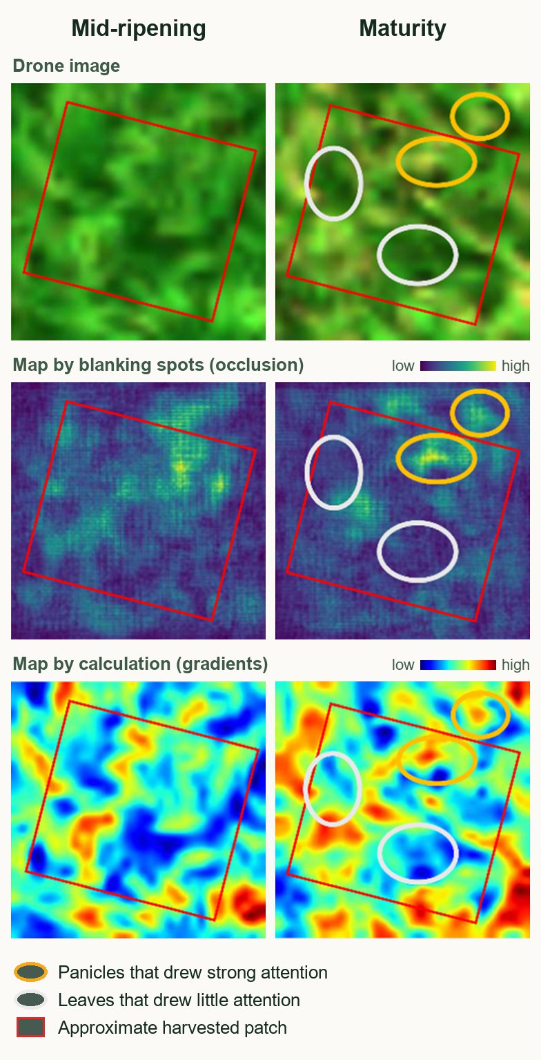
The AI's focus on panicles at maturity fits the two findings above. Previous studies report that red edge light responds to panicles once they emerge and their color and shape change. A slightly wider square also takes in panicles that droop outward, which likely helped accuracy.
Toward more accurate and trustworthy yield predictions
This study shows that when drones and CNNs are used to predict rice yield, the input images should be matched to the growth stage. Near harvest, light that includes red edge and a square slightly wider than the harvested patch work well.
More accurate predictions could help produce better yield maps, which show where a field yields more and where it yields less. Knowing the yield in advance supports farmers' decisions.
The XAI results matter too. When an AI attends to places that make sense in terms of how rice grows, we can trust its predictions more.
How accurate is it?
Our R² values (0.347 to 0.492) are lower than those of drone and CNN studies on soybean and wheat, but similar to those of earlier rice studies. They are far higher than those obtained with vegetation indices, which are simple greenness measures calculated from reflected light. Our data span three years, five varieties, and a wide range of yields, and we consider this accuracy sufficient for comparing image conditions.
What we do not know yet
These results come from rice. We have not yet tested whether the same conditions work for crops such as maize and wheat. Their grain heads droop less and change color differently, so the best conditions may also differ.
We also imaged only two stages. Other studies report that combining images from more stages improves accuracy, but each extra flight costs time and money. Finding the right balance is a task for future work.
Next steps
Checking where an AI looks can also reveal weaknesses in the current model and point to improvements. Next, we want to build more trustworthy models that, from an agronomic point of view, look at the right parts of the plant.
Glossary
- Panicle
- The grain head of a rice plant. It is the branched cluster at the top of a stem where the grains form, and it bends down as the grains fill.
- Multispectral camera
- A camera that records light separately for each color, or wavelength. It can also capture near-infrared light, which our eyes cannot see.
- Near-infrared (NIR) and red edge
- Near-infrared light lies just beyond red, is invisible to our eyes, and tracks the amount of leaves and the size of plants well. Red edge is the band between red and near-infrared.
- Convolutional neural network (CNN)
- A type of AI, and a kind of deep learning, that scans an image with small filters and combines the patterns it finds over many layers.
- Explainable AI (XAI)
- Methods that show, in a form people can understand, why an AI gave its answer. Here we used XAI to map where the AI looked in each image.
- Heat map
- A map that shows values as colors or brightness. In this study, brighter or redder areas are where the AI focused more.
- Occlusion sensitivity and gradient method
- Two ways to find where an AI looks. Occlusion sensitivity blanks out spots one at a time and watches the prediction change. The gradient method calculates how sensitive the prediction is to a small change at each point.
- Mid-ripening and maturity
- Ripening is the period after heading when the grains fill. In this study, mid-ripening means about three weeks after heading, and maturity means around harvest.
- Coefficient of determination (R²)
- A number that shows how well predictions match measurements. The closer it is to 1, the better. A value of 0 means the predictions are no better than always guessing the average.
- Cross-validation
- A way to test a model on data it has not learned from. Each group of data takes a turn as the test set, and the results are averaged.
About the paper
Tomoaki Yamaguchi, Taiga Takamura, Takashi S.T. Tanaka, Taiichiro Ookawa & Keisuke Katsura (2025). A study on optimal input images for rice yield prediction models using CNN with UAV imagery and its reasoning using explainable AI. European Journal of Agronomy, 164, 127512. https://doi.org/10.1016/j.eja.2025.127512
The paper is open access, so anyone can read it free of charge. It is published under the CC BY-NC 4.0 license, which allows non-commercial reuse with credit. Some figures on this page were made from the paper's figures under this license.