04 — Publications / Explainer
Why do actual rice yields fall short of
the ceiling the weather sets?
Five decades of a Philippine rice experiment, read with a crop model and machine learning
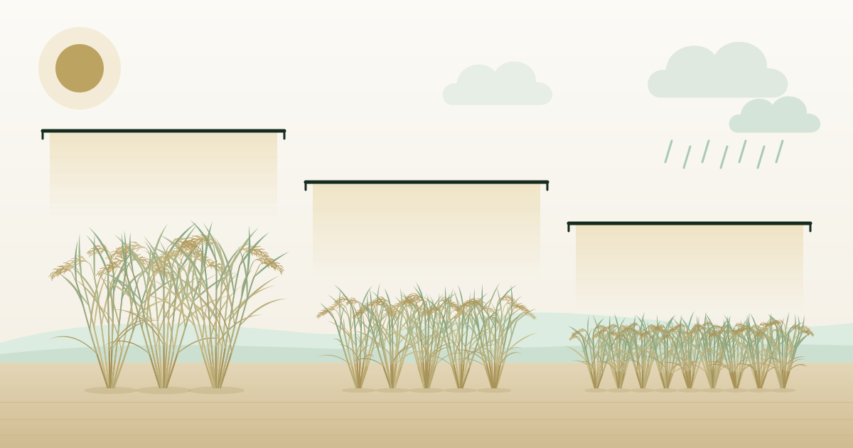
Every rice field has a ceiling, the largest harvest that the season's weather and the variety allow. Using about 50 years of records from a Philippine trial that grows rice three times a year, we measured how far real yields fell below it. In the wet seasons, fields produced only about half of what was possible, and disease and aging varieties were major reasons why. Even with both removed in our calculations, yields reached only 63 to 69% of the ceiling, short of the widely used 80% benchmark.
Key points
- Even at the two highest nitrogen levels, harvests reached about 65% of the ceiling in the dry season, but only about 52% and 47% in the early and late wet seasons.
- Nitrogen fertilizer had the strongest effect across the seasons. Tungro, a virus disease, widened the gap in the dry season, and aging varieties widened it in the late wet season.
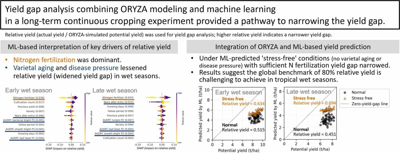
- With disease and variety aging removed, predicted yields reached 63 to 69% of the ceiling. The global 80% benchmark appears hard to reach in tropical wet seasons.
How much more could the same field produce?
How much more rice could the same field produce? The answer is a starting point for keeping food supplies secure.
Rice yields have a ceiling, called the potential yield. It is the harvest a variety would give with plenty of water and nutrients and no damage from pests or disease. It depends on the season's sunlight and temperature and on the traits of the variety.
Real fields produce less, and the difference is called the yield gap. We expressed actual yield as a percentage of potential yield, called the relative yield (Figure 1). The higher it is, the smaller the gap. Knowing the size of the gap and its causes shows which fixes deserve attention first.
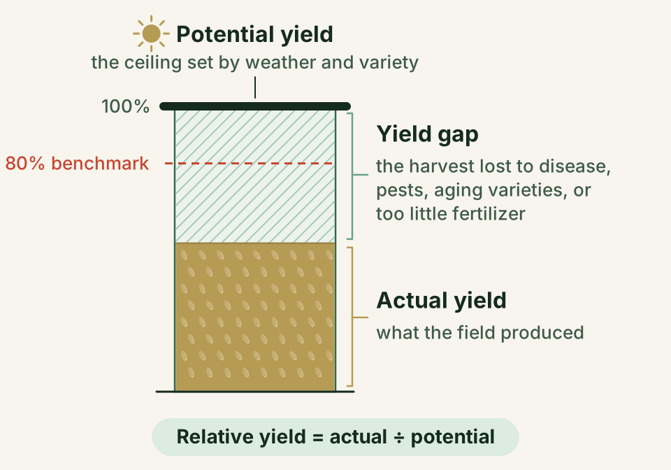
A real field cannot be expected to reach 100% of its ceiling. Some pests and disease always remain, the weather varies, and management has limits. So about 80% of the ceiling is widely used around the world as the benchmark for a well-managed field.
Most yield gap studies so far have looked at farmers' fields. Long-term experiments keep consistent records on the same field for decades, which makes them ideal for finding out why yields changed. Yet their records had rarely been used to study yield gaps.
Reading 50 years of records in four steps
A field that grows rice three times a year
Our study used the Long-Term Continuous Cropping Experiment at the International Rice Research Institute (IRRI) in Los Baños, the Philippines. It is the world's longest-running trial of irrigated rice grown three times a year.
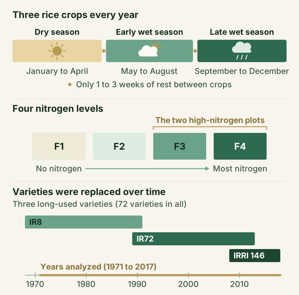
Rice is grown in the dry season (January to April), the early wet season (May to August), and the late wet season (September to December), with only one to three weeks of rest between crops. The field has four nitrogen fertilizer levels, from F1, which receives none, to F4, which receives the most.
Varieties were regularly replaced with newer ones that resist pests and disease better, and 72 were used from 1968 to 2017 (Figure 2). We analyzed the records from 1971 to 2017, because the weather data before 1971 fluctuated irregularly.
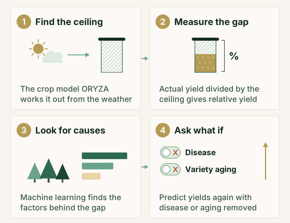
We worked through the four steps shown in Figure 3.
A crop model computes the ceiling
We computed the potential yield with ORYZA, a crop model. A crop model is a computer program that simulates how a crop grows, day by day, from the weather. Here it assumed plenty of water and nutrients and no pests or disease.
We ran it for IR8, IR72, and IRRI 146, three varieties used in the trial for more than ten years, and took their average as the potential yield for each season in each year. Weather data came from JRA-55, a continuous reconstruction of past weather from the Japan Meteorological Agency, adjusted to local measurements.
Relative yield measures the gap
Dividing actual yield by potential yield gave the relative yield. We focused on F3 and F4, the two highest nitrogen levels, averaged across varieties. We also calculated the relative yield of the best variety and fertilizer combination of each year.
Machine learning looks for causes
Next, we used machine learning to find out why relative yield rose and fell from year to year. Machine learning lets a computer learn patterns from many records. We used a method called random forest, with a separate model for each season.
The models drew on clues such as the nitrogen rate, disease risk, the variety, variety aging, and the number of crops grown since the trial began. Variety aging is the number of years since a variety entered the trial. A method called SHAP measured how much each factor pushed the predictions up or down. We checked each model by predicting years it had not seen.
Disease levels were not recorded consistently over the 50 years. Instead, we used EPIRICE, a model that estimates from the weather how easily five diseases spread. They were leaf blast, brown spot, bacterial blight, sheath blight, and tungro. The model's estimates are weather-based risks, not damage seen in the field.
Asking what if
Finally, we used a yield prediction model built with machine learning in our earlier study (2025). It predicted yields with disease risk set to zero, with variety aging set to zero (as if every variety were new), and with both at zero. We then compared the predicted yields with the potential yield. The case with both at zero comes close to the stress-free world that ORYZA assumes.
The size and causes of the gap differed by season
In the wet seasons, fields reached only about half of the ceiling
The potential yield was highest in the dry season, at 10.41 metric tons per hectare on average. It was 8.63 tons in the early wet season and 7.15 tons in the late wet season.
At F3 and F4, actual yields averaged 6.52 to 6.86 tons in the dry season, 4.39 to 4.50 tons in the early wet season, and 3.28 to 3.38 tons in the late wet season (Figure 4). These correspond to relative yields of 64.5%, 51.7%, and 46.7%.
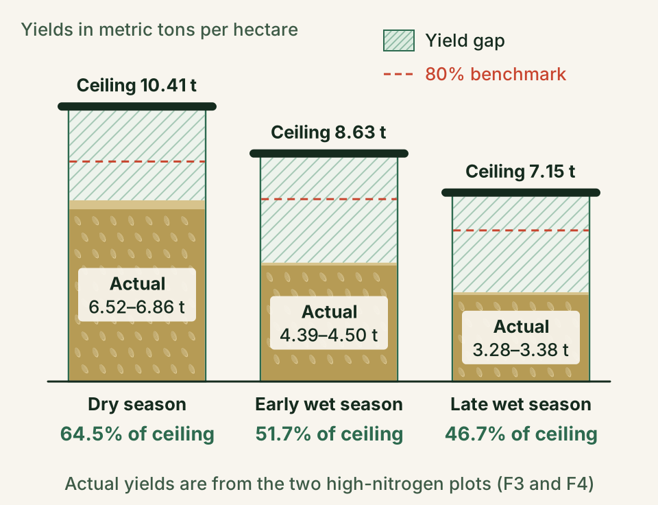
The best variety and fertilizer combination of each year showed the same pattern, at 72.6%, 60.4%, and 56.0%. Even in the dry season, only 23.4% of years reached 80%. In the wet seasons, no year did, apart from a few in the early wet season.
The ceiling itself changed little from year to year, so the gap moved mainly with actual yield. Relative yields also stepped up by 8.0 to 15.0 percentage points in the early 1990s. This was a single step, probably from better crop management at that time, rather than a slow, steady rise.
Each season had its own causes
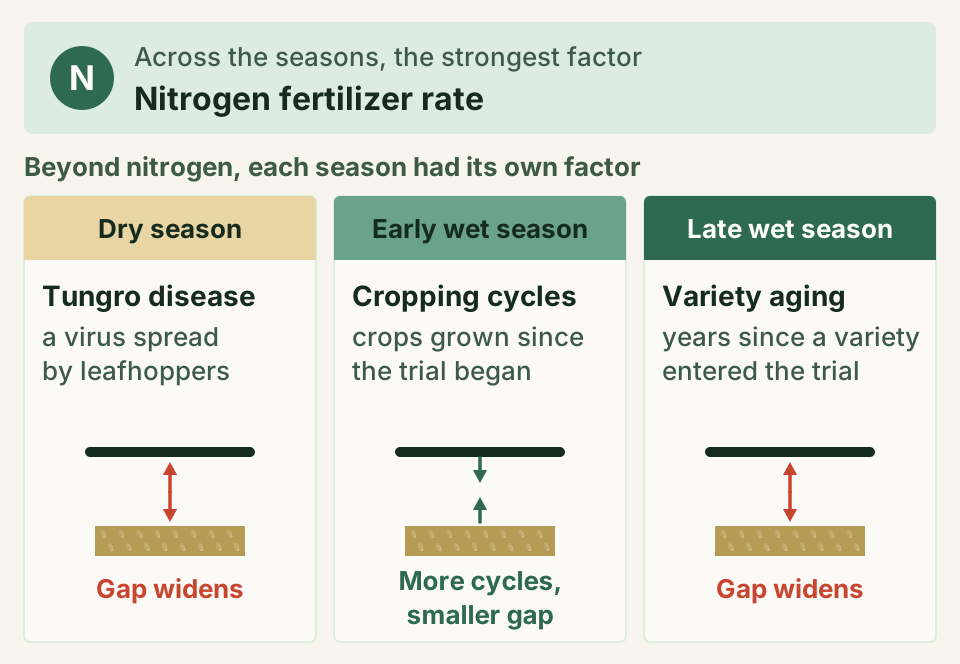
Across the seasons, the machine learning analysis found that the nitrogen rate had the strongest effect on relative yield (Figure 5), as studies in farmers' fields have long shown. Beyond nitrogen, each season had a factor of its own.
In the dry season, tungro widened the gap. This virus disease is spread by green leafhoppers, and in this trial it came from nearby fields planted at different times. It can cut yields without clear symptoms by reducing the number of grains that fill. Its damage also tended to grow with the nitrogen rate, which fits reports that nitrogen makes leaves lush and inviting to leafhoppers.
In the early wet season, the more crops had been grown since the trial began, the smaller the gap.
In the late wet season, variety aging widened the gap and ranked second in importance after nitrogen. Earlier studies have shown that when a variety stays in use for many years, pests and pathogens change and its resistance gradually weakens.
Removing disease and variety aging narrowed the wet-season gap
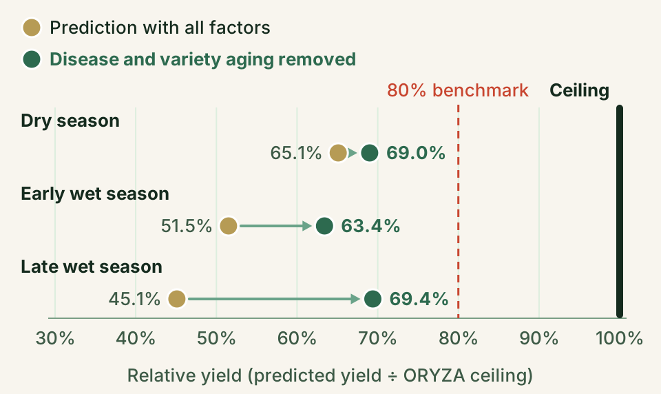
With all factors included, the predicted relative yields were 65.1%, 51.5%, and 45.1% for the dry, early wet, and late wet seasons (Figure 6), close to the values observed at F3 and F4. With disease and variety aging removed, they rose to 69.0%, 63.4%, and 69.4%. The gains were largest in the wet seasons.
In the wet seasons, these predictions now rose and fell in step with the ORYZA ceiling from year to year. So the wet-season gap came mainly from two things ORYZA leaves out, disease and the turnover of varieties. Even so, no season reached 80%.
A mismatch remained in the dry season
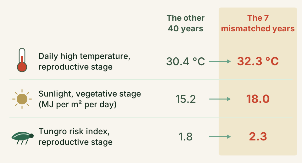
In the dry season, even these predictions did not move with the ORYZA ceiling. We found seven cases in which the ceiling was at least 4.1 metric tons per hectare above the prediction, and all of them were in the dry season.
In those years, the daily high temperature in the reproductive stage, when the plant forms its grain heads, averaged 32.3 °C, against 30.4 °C in the other years. Sunlight was also stronger, and tungro risk was higher (Figure 7). ORYZA may not fully capture how heat affects photosynthesis, but this study cannot tell whether the cause lies in the model, the input data, or elsewhere.
Targets that fit the season, and ways to narrow the gap
Around the world, 80% of the ceiling has served as the benchmark for a well-managed field. Yet in the wet seasons of this trial, yields reached only 63 to 69% even with disease and variety aging removed. In the humid tropics, especially in the wet seasons, even staying above about 70% of the ceiling may be difficult.
In the dry season, yields averaged 77% of the ceiling after management was revised in the 1990s, close to the benchmark. We think targets should fit each season and place, rather than follow one global number.
Ways to narrow the gap
In the wet seasons, replacing varieties more often and strengthening disease control could help. In the dry season, controlling tungro is key. Proven measures include resistant varieties, planting at the same time as neighboring fields, and fallow periods that reduce the sources of the virus. Adjusting nitrogen use along with disease control might narrow the gap further.
The best variety and fertilizer combination of each year beat the high-nitrogen average by 6.5 to 10.0 percentage points in relative yield. Choosing varieties well, along with good fertilizer management, is a practical way to narrow the gap.
A crop model shows the ceiling the weather allows, and machine learning shows what holds real fields below it. Together, they let us diagnose the gap season by season.
What we do not know yet
- The results come from one long-term trial of intensive, irrigated rice in the tropics.
- The disease numbers are weather-based risks, not measured damage.
- The ORYZA ceiling leaves out disease, variety aging, and nitrogen shortage. For the early wet season, our earlier study suggested that soil nitrogen may rise as temperatures climb early in the season.
- The cause of the dry-season mismatch, and how much of the remaining gap can be closed, are still open questions.
Next steps
We think a combined approach would work well. ORYZA would set each season's ceiling, with disease risk at each growth stage and variety turnover built in. Machine learning would then estimate the gap that remains. In the dry season, heat during the reproductive stage and the response to sunlight deserve a closer look.
Glossary
- Potential yield
- The most a crop can yield with plenty of water and nutrients and no pests or disease. It depends on the weather and the variety.
- Yield gap
- The difference between potential yield and actual yield.
- Relative yield
- Actual yield as a percentage of potential yield. The higher it is, the smaller the yield gap.
- Crop model (ORYZA)
- A computer program that simulates crop growth and yield from daily weather and other inputs. ORYZA is a model for rice.
- Machine learning (random forest)
- Methods that let a computer learn patterns from data. Random forest averages the answers of many simple yes-or-no decision trees.
- SHAP
- A method that shows how much, and in which direction, each factor moved a prediction.
- Variety aging
- The number of years since a variety entered the trial. Over time, a variety can lose resistance to pests and disease.
- Tungro
- A virus disease of rice spread by green leafhoppers. It can lower yields even without clear symptoms.
- EPIRICE
- A model that estimates from the weather how easily rice diseases spread, giving a risk index for each growth stage.
About the paper
Tomoaki Yamaguchi, Ando Mariot Radanielson, Olivyn Angeles, Keisuke Katsura & Kazuki Saito (2026). Understanding rice yield gaps with crop modeling and machine learning in a long-term continuous cropping experiment. Field Crops Research, 342, 110477. https://doi.org/10.1016/j.fcr.2026.110477
This open access paper is free for anyone to read. It is published under the CC BY 4.0 license. Figure 8 is reproduced from the paper, and Figures 4, 6, and 7 were drawn from values reported in it.