Orthoimages and DSMs (Digital Surface Models) from a drone hold a lot of information about a crop's condition. If you compute features such as vegetation indices and plant height from them, and pull out a single value for each field polygon, you can compare and analyze growth plot by plot. This page walks through the whole flow in the free GIS software QGIS, from opening the data, to computing features, to summarizing them per polygon and exporting to CSV, step by step.
What you need (all free)
- QGIS — free GIS software from qgis.org
- Orthoimage and DSM — a .tif orthoimage and Digital Surface Model built from drone imagery
- Polygons — vector data dividing the field into plots (.shp or .gpkg)
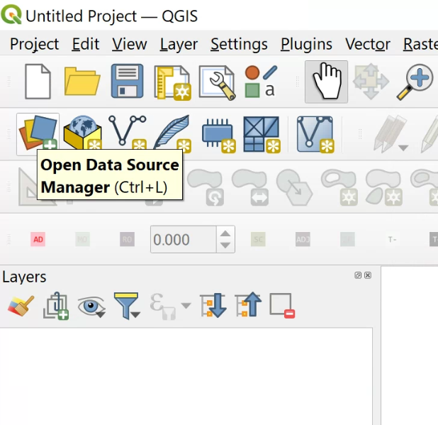
You load data into QGIS from the "Data Source Manager" (the icon at the top-left of the toolbar, or Ctrl+L). Switch tabs depending on the type of data you are opening.
Open the orthoimage and DSM (raster)
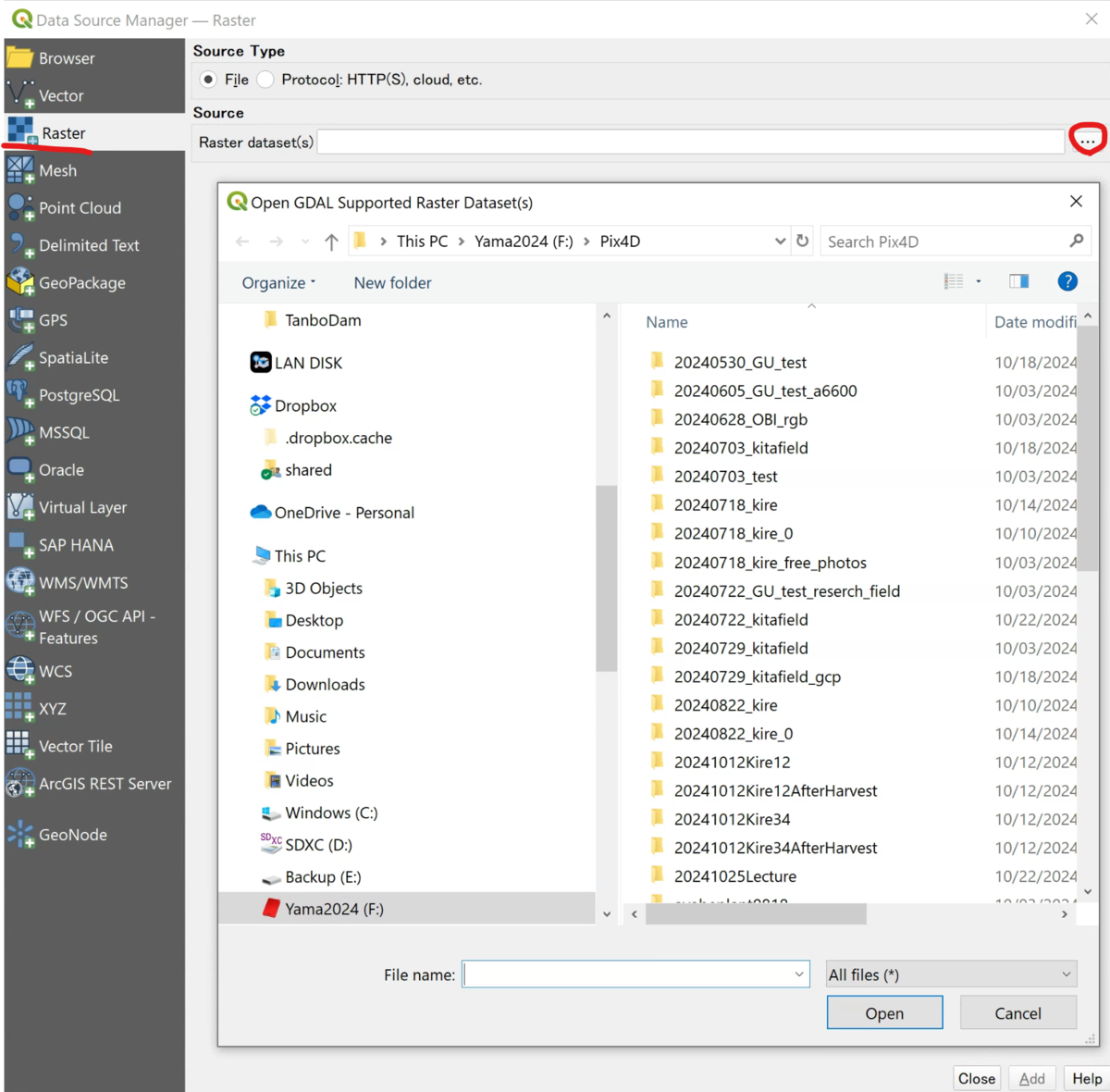
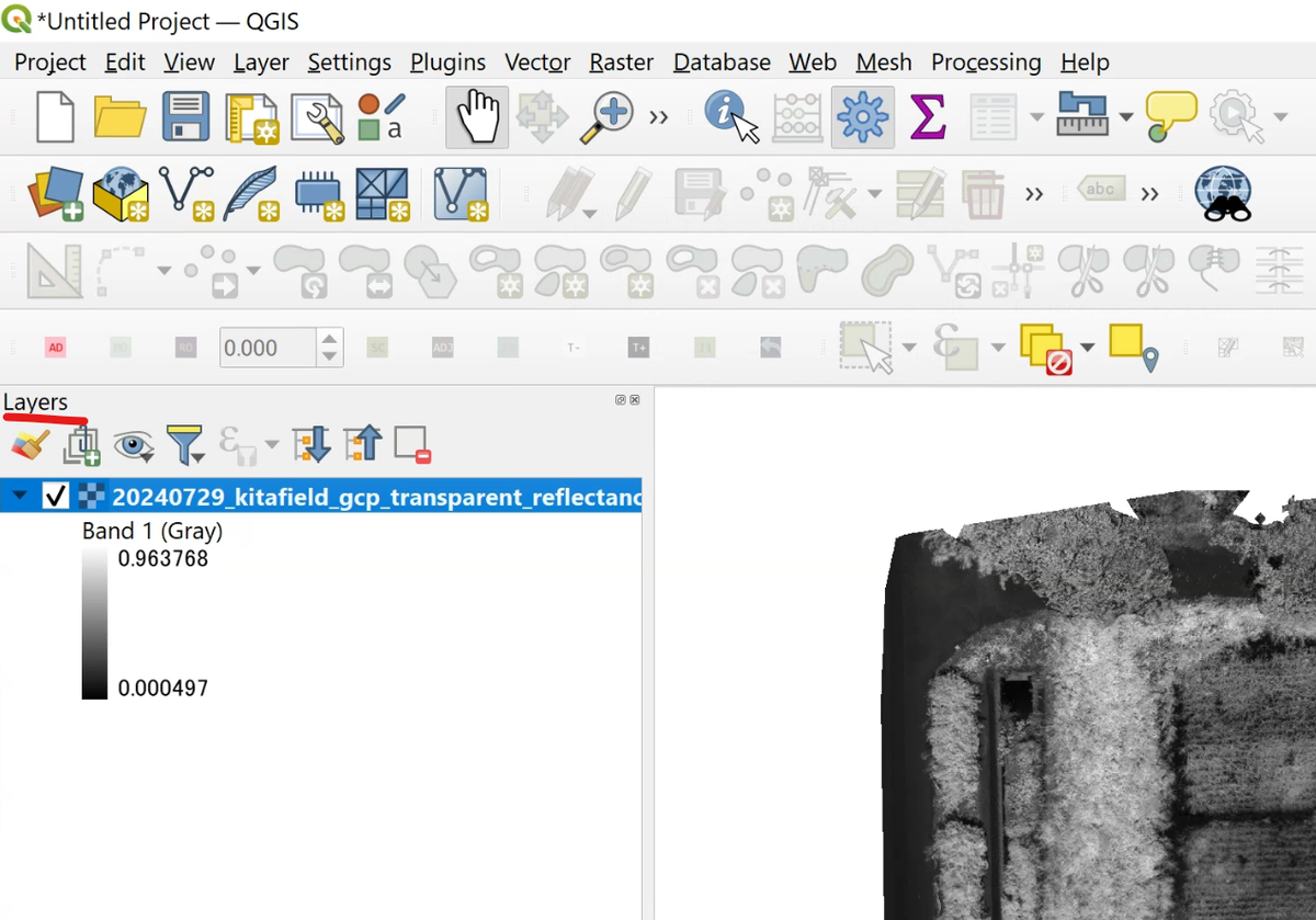
On the "Raster" tab, choose the .tif orthoimage or DSM and click "Add." If the image appears on the map, it loaded successfully.
Open the polygons
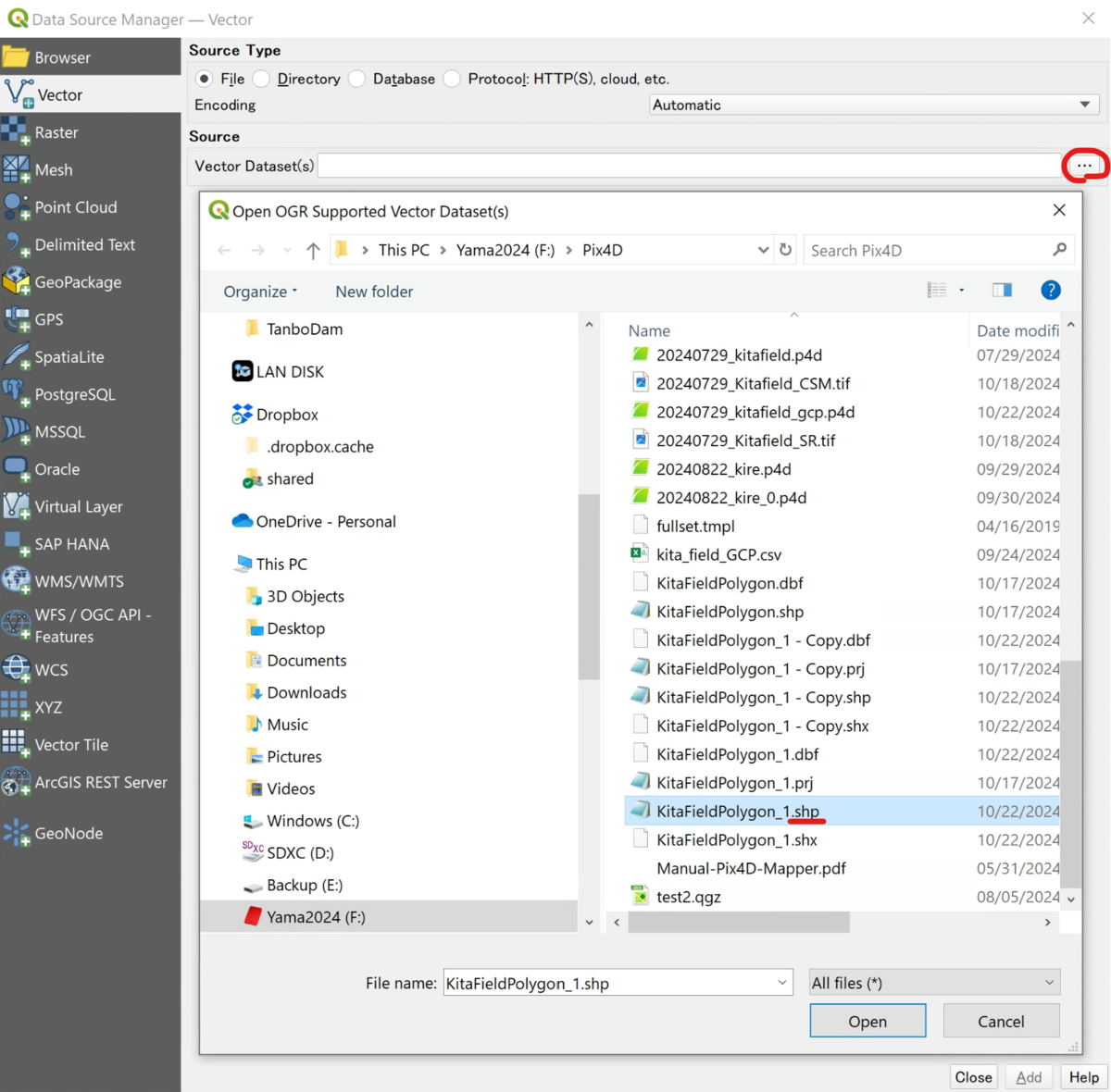
From the "Vector" tab, add the plot polygons (.shp or .gpkg). They appear layered over the orthoimage.
Open a CSV or ground control points (GCP)
A CSV that carries coordinates (such as ground control points) is opened from the "Delimited Text" tab. Set the encoding to UTF-8, the delimiter to comma, and check "First record has field names" and "Detect field types." If it has coordinates, choose "Point coordinates" under Geometry Definition and specify the X and Y (and Z, if any) fields.
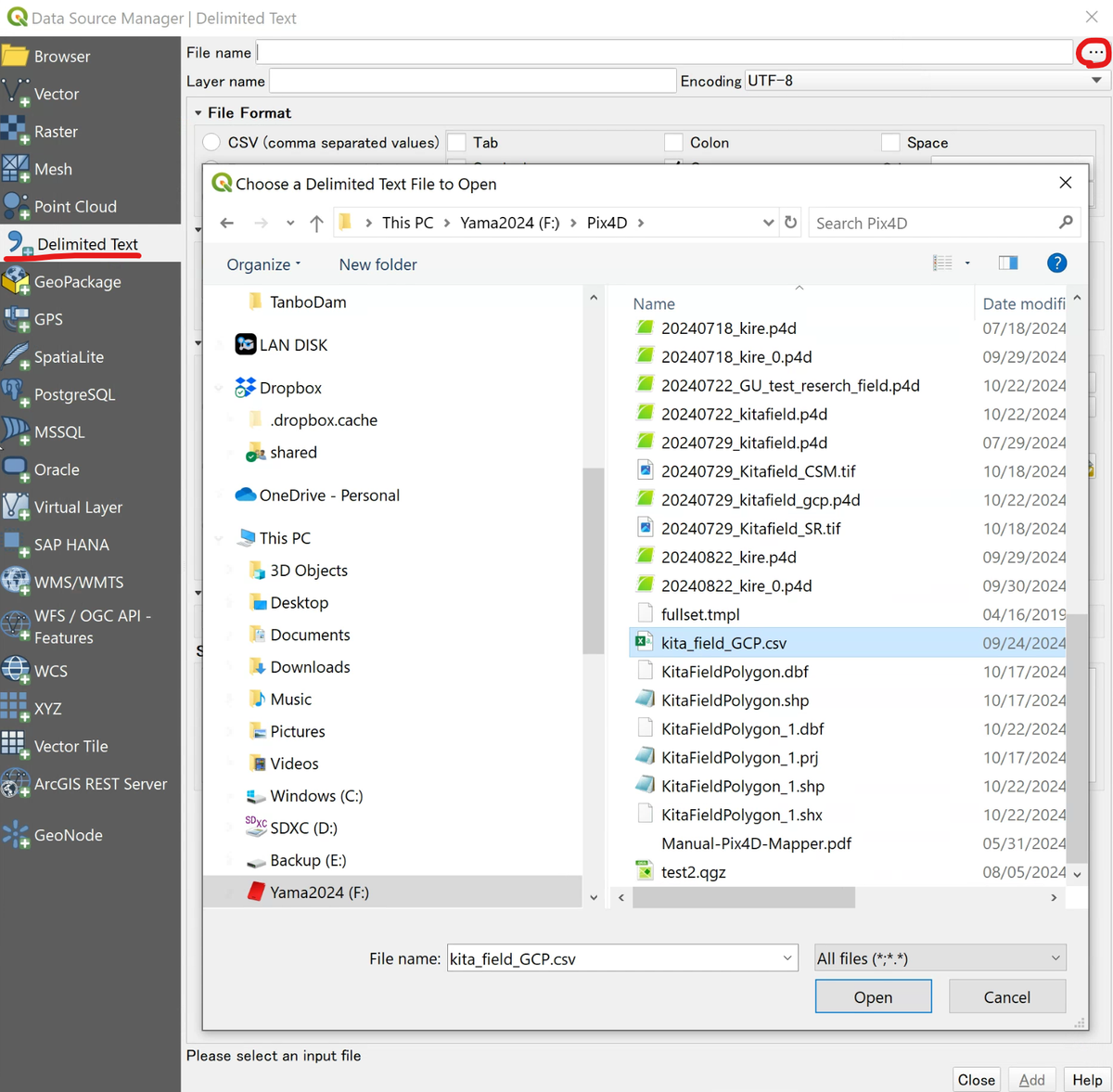
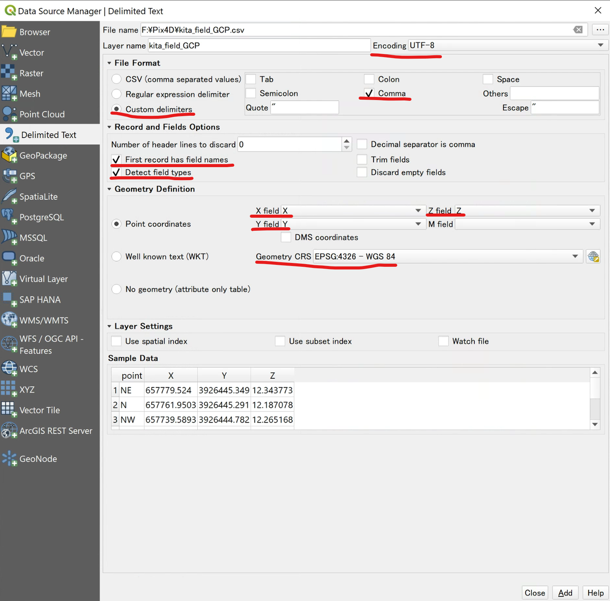
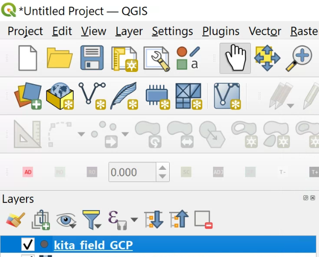
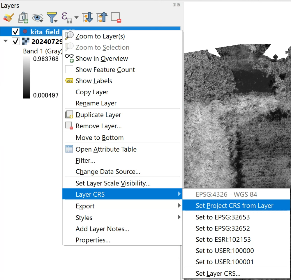
If the coordinate reference system (CRS) of the points does not match, right-click the layer and set it (for example, "Layer CRS → Set Project CRS from Layer," such as EPSG:32653). If the points are too small to see, adjust their size and color in Properties → "Symbology."
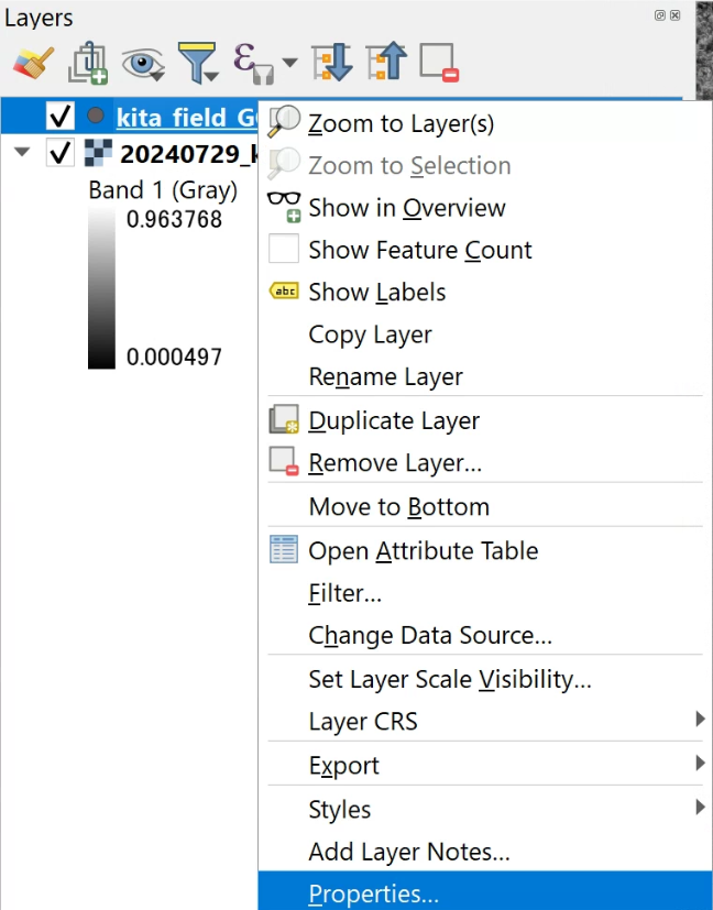
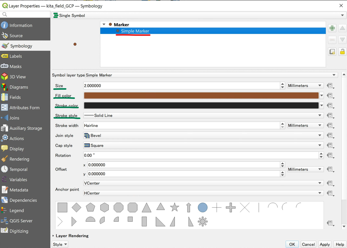
For a CSV that has attributes only, with no coordinates (a table of variety names, replication numbers, and so on), choose "No geometry (attribute only table)" under Geometry Definition. You will join it to the polygons in the next step.
When plot attributes (variety, replication, and so on) live in a separate CSV, join them to the polygons using a shared column (for example, fid). Right-click the polygon layer and open "Properties → Joins," then click "+". Set the attribute CSV as the "Join layer," set the shared column as both the "Join field" and "Target field," check only the attributes you need, and click "OK."
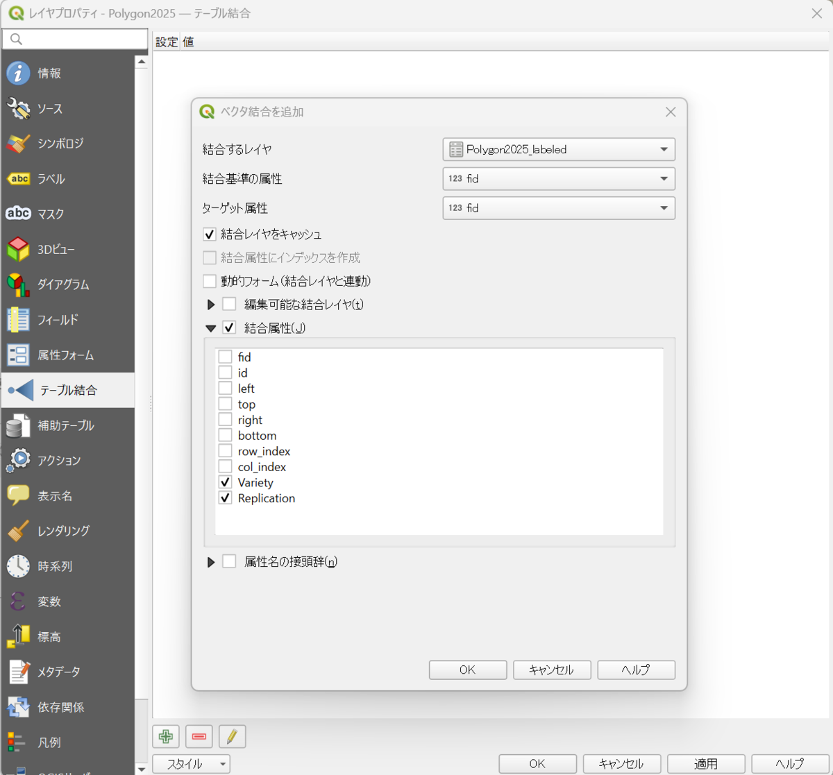
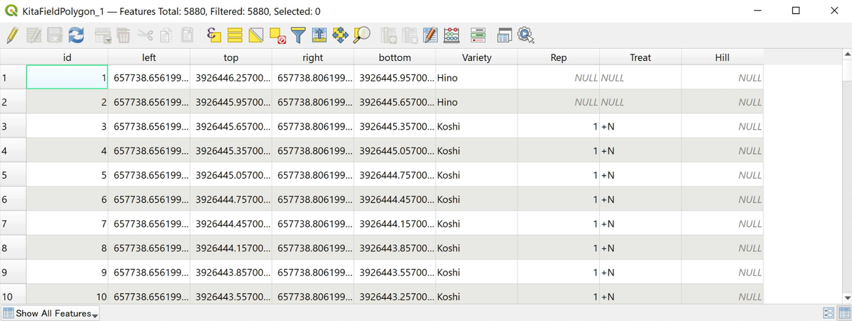
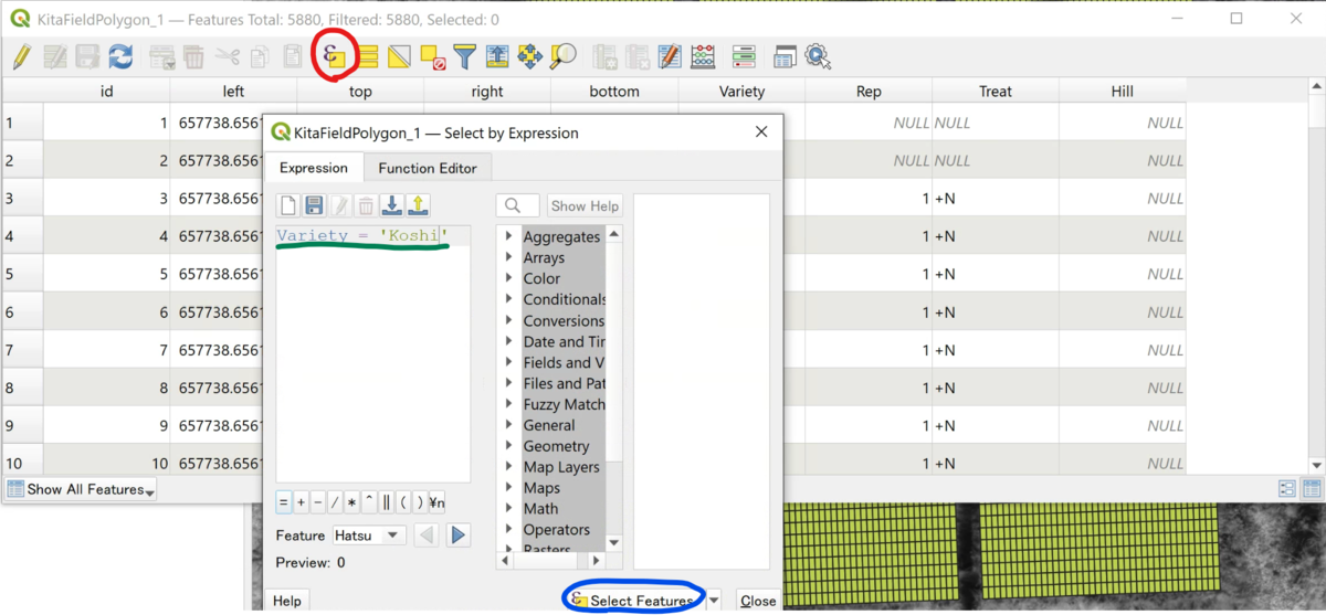
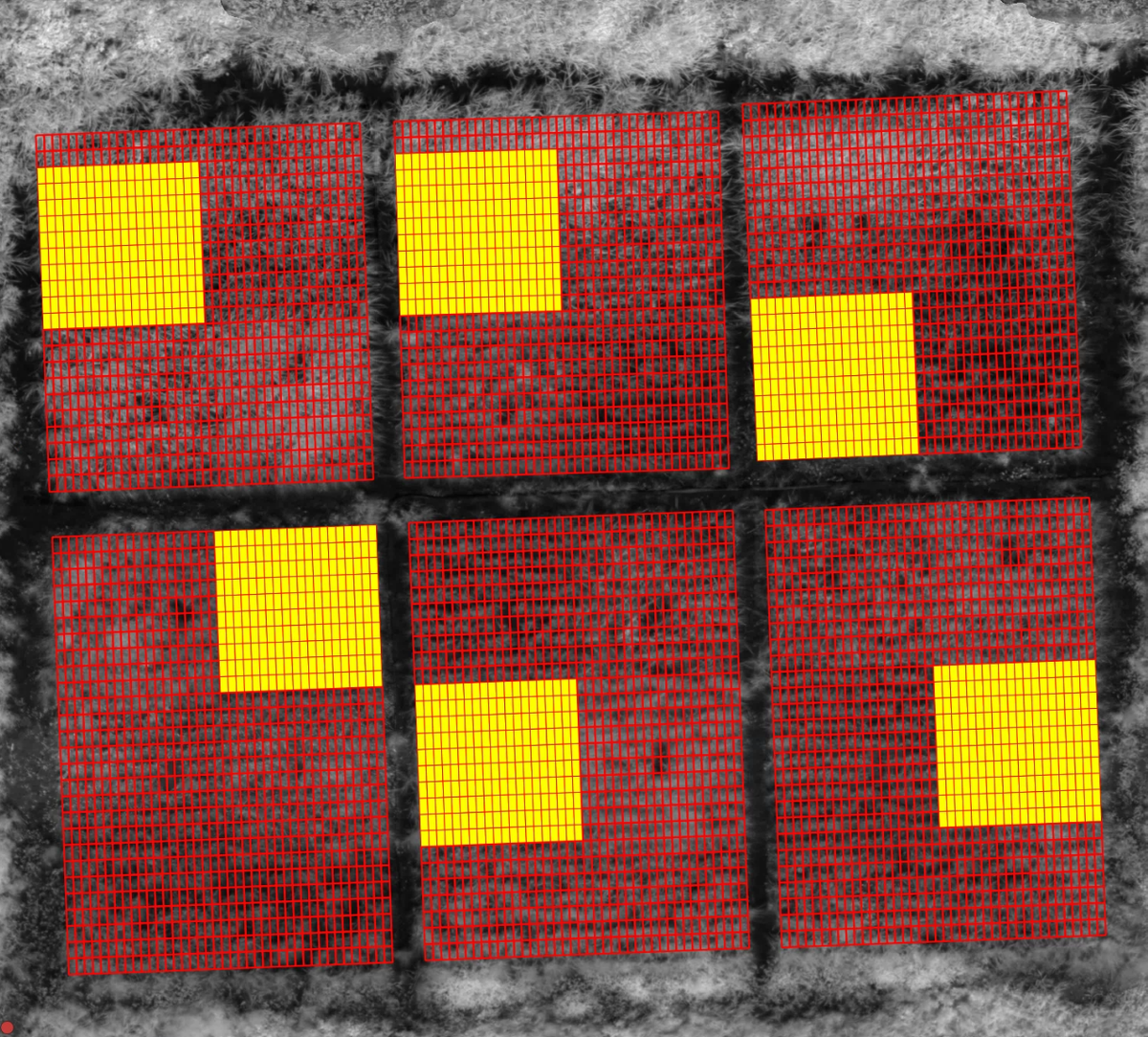
Once joined, confirm that the attributes are linked to the right polygons. Open the polygon's attribute table and you will see the joined columns (such as variety) added. Using "Select by Expression," you can enter a condition like Variety = 'Koshi' to highlight only the matching plots on the map.
With labels, you can display the variety name or number directly on each plot. Check on the map that the plots are laid out the way you intend.
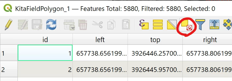
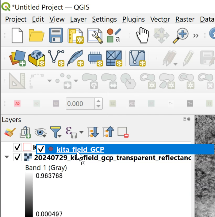
A few basics make the work much smoother. Drag to pan, use the mouse wheel to zoom, and toggle the checkboxes in the "Layers" panel to show or hide layers. Layers higher in the list are drawn in front, so reorder them to control what overlaps what.
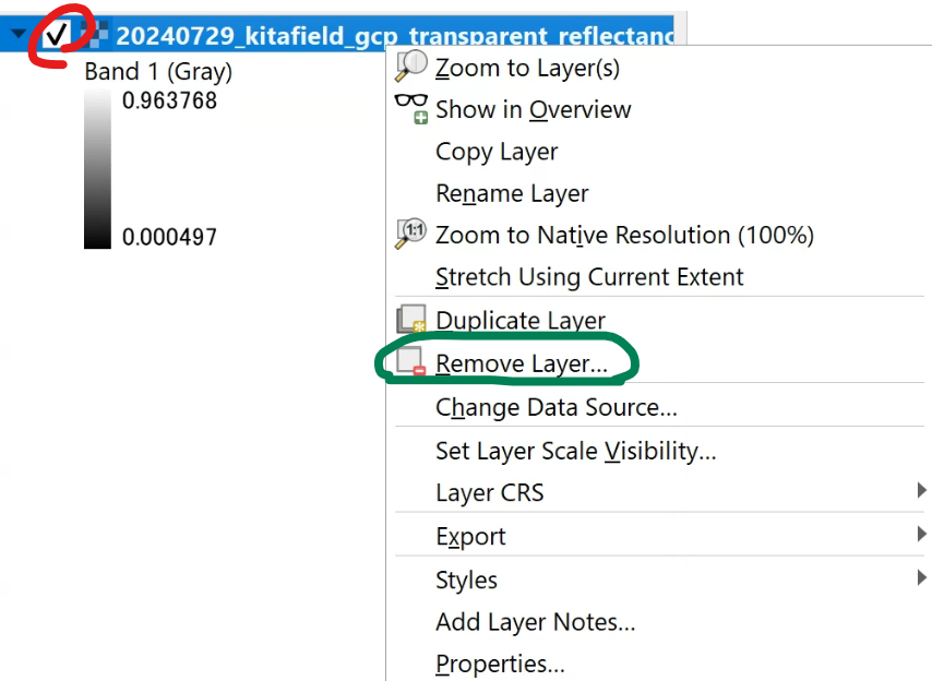
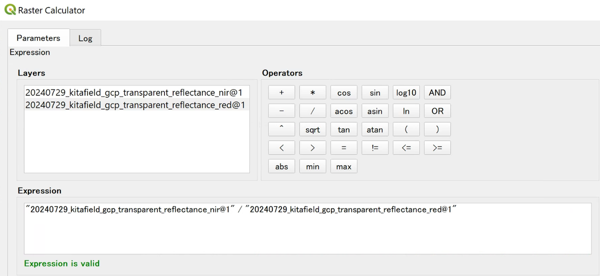
Compute features with the "Raster Calculator" ("Processing → Toolbox → Raster analysis → Raster calculator"). In the expression field, write a formula that combines the bands you want. For the simple ratio (SR) index, for example, divide the near-infrared (NIR) band by the red (Red) band.
"(NIR band)@1" / "(Red band)@1"
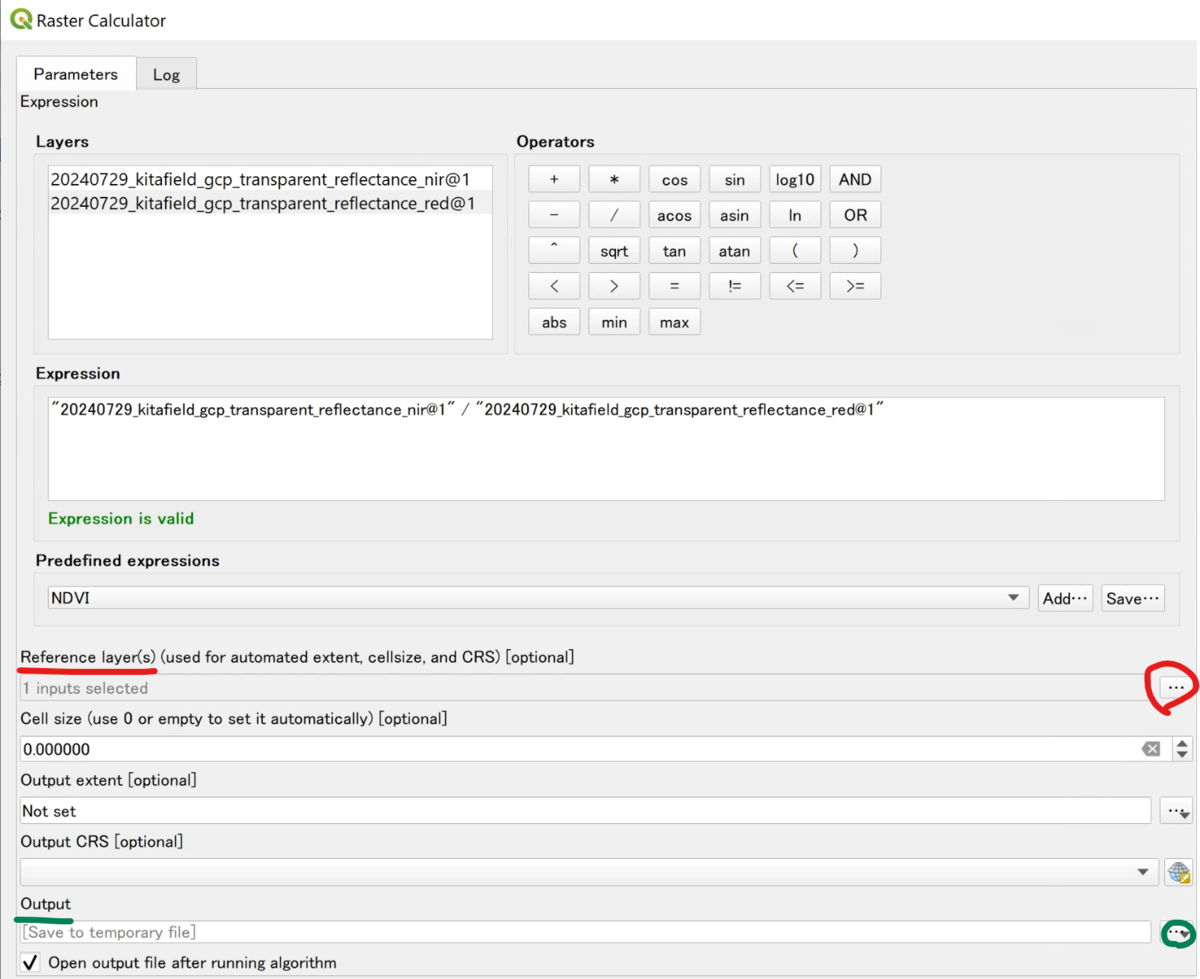
For plant height, subtract a ground-only DSM (baseline) from the DSM taken when the crop is grown.
"(growth-stage DSM)@1" - "(ground DSM)@1"
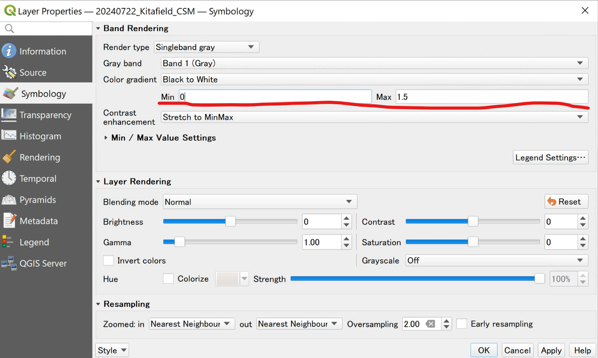
If the result looks too dark to read, adjust the display minimum and maximum (Min / Max) in Properties → "Symbology" to make the distribution easier to see.
Now reduce each feature to a single number per plot. Open "Processing → Toolbox → Raster analysis → Zonal statistics," set the plot polygons as the input layer and the feature image as the raster layer. Check "Mean" among the statistics and run it, and you get the mean of the pixels inside each polygon, plot by plot.
You can save the output as CSV. Leave "Open output file after running algorithm" unchecked so you do not pile up extra layers, which makes the next join easier. Repeat the same step for each feature: vegetation index, plant height, texture, and so on.
Join the CSV from zonal statistics to the polygons with the same "Joins" as in Step 2, and each plot lines up in one table with "variety, replication, vegetation index, plant height, ...". Finally, right-click the polygon and choose "Export → Save Features As," set the format to CSV, and write it out.
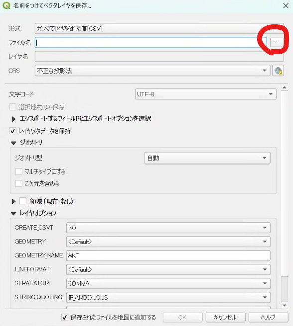
You can leave "Add saved file to map" unchecked. Open the exported CSV in Excel and resave it as .xlsx, and it is ready for statistical analysis and plotting.
At this point you have turned drone imagery into a single table of features, one row per plot. Analyze that table and you can compare growth across varieties and treatments in numbers. Start with a single feature to learn the flow, then add more as you go: vegetation indices, plant height, texture, and beyond.